WXB-006
[Paper] Native Sparse Attention: Hardware-Aligned and Natively Trainable Sparse Attention
来自 Deepseek 的大作 NSA,同时也是 ACL2025 的 best paper。
- tl;dr: 做了关于 sparse attention 的算法改进,同时考虑了对大规模模型的 efficiency。实验结果上,甚至比原先的 full attention 有更低的 loss 和更好的 reasoning performance,并且在较长的 context 上提速 10 倍。
Background: Sparse Attention
LLM 做的任务可以分为两种:compute-bound 和 memory-bound。比如 LLM inference,分为 prefilling 和 decoding phase:前者是同时处理所有输入获得 hidden layer 的 KV;后者是 next-token prediction 生成输出。Prefilling 主要在做大规模矩阵乘法,是 compute-bound;decoding 的 bottleneck 在于 KV-cache,属于 memory-bound。
现在的编程任务或者阅读文献都是重在 prefilling,用户对话重在 decoding,所以工业上来说这两方面都要优化。
- Grouped-Query Attention (GQA): 将 attention heads 分为若干个 group,每个 group 用同样的 KV-cache。
为了在做到 sparse attention 的情况下没有 performance degradation 并且确保 efficiency,我们需要:
- Sparse attention 架构需要同时用到 training 和 inference,否则会有误差。
- Block 的选择首先要远小于 full attention,其次要精准的 cover attention weight。
- 选择 block 的时候不能出现 non-trainable components。典型的反例是 ClusterKV (把 KV value 做 k-mean clustering)。这样还需要加各种 balance loss,必然会 distract。
- Block 的选择需要尽量保证连续化,否则在 GPU 上无法优化。这里的 metric 是 arithmetic intensity: number of arithmetic operations 与 memory access 之比。
Native Sparse Attention (NSA)
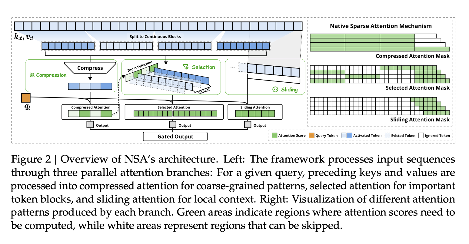
这张图意思到了,但是有一些细节没表达清楚。NSA 的方法是,序列每个位置 $t$,我们把 attention output $o_t$ 的计算分为三个部分:Token Compression, Token Selection, 以及 Sliding Window。假设我们分别得到了三个 output $o_t^{i}$ ($1\le i\le 3$), 最终的 output 是
\[o_t=\sum_{i} g_t^{i}o_t^{i},\]其中 $g_t^i\in [0,1]$ 是 scalar,使用输入的 feature 过 MLP 得到。
三个部分分别用不同的 $K$ 和 $V$,但是共享 $Q$。
1. Token Compression
包含超参 $l>d$,其中 $d\mid l$。将连续 $l$ 个 token(称为一个 block) 合并为一个(使用带 positional embedding 的 MLP)。相邻两个 block 移动 $d$ 位,保证 overlap,这样学出来更加 smooth。
形式化地,对非负整数 $i$,把 $k_{i\cdot d}$ 到 $k_{i\cdot d+l-1}$ concat (w/ PE) 然后过 MLP $\varphi$,得到新的 key $\tilde k_i$:
\[\tilde k_i=\varphi(k_{i\cdot d\ :\ i\cdot d+l}),\quad i\le \dfrac{t-l}{d},\]然后将 $q_t$ 对这些 $\tilde k_i$ 做 attention。
实践上取 $d=16$, $l=32$,这样会把序列长度变为原来的 $1/16$。Intuition 是用 MLP 来“总结”一段序列的 feature。
2. Token Selection
包含超参 $l’$,还是要满足 $d\mid l’$;以及 $n$。前一种方法的 attention 毕竟是总结出来的 feature,不太准确;所以对于那些 attention score 最高的 $n$ 个 block (长度为 $l’$),我们需要把它拆开做更细的 attention(注意这里这些长 $l’$ 的 block 是不交的)。
这样选择的理由是:
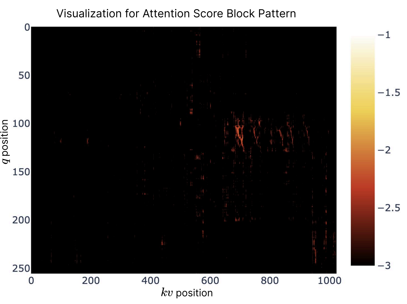
- visualizing attention map 发现 attention score 高的点附近的 score 也会跟着高;
- 假如 $l’$ 被 kernel block size 整除,计算就很迅速。
这里一个简化计算图的方法是,我们直接用第一部分算出来的 block attention score。但问题是 $l<l’$。解决办法是启发式地用连续 $l$ 个 token 的 score 来预测连续 $l’$ 个 token 的 score。
假设第一部分算出来的 score 是 \(\mathbf {p}_t=\text{softmax}(q_t^T[\tilde k_1,\tilde k_2,\cdots]),\)
那么我们定义一个 $d$-block 的 score 等于所有包含它的 $l$-block score 之和;再定义 $l’$-block 的 score 等于所有里面 $d$-block 的 score 之和。写成公式就是 \(\mathbf{p}^{\text{select}}_t[j]=\sum_{m=0}^{l'/d-1}\sum_{n=0}^{l/d-1} \mathbf p_t[\dfrac{l'}{d}\cdot j-m-n].\)
然后利用这个 $\mathbf{p}_t^{\text{select}}$ 来选出前 $n$ 个块,组成长为 $n\cdot l’$ 的 key sequence 再求一次 attention。
实践上取 $l’=64$, $n=16$。这样这个部分会固定选出 $1024$ 个 token。
- 细节:如果要用 GQA,那么同样的 group 应该注意到相同的 key,所以我们强制对这个 group 的 $p$ 取平均来保证选出相同的 token。
3. Sliding Window
这个部分和 common practice 一致。取 $w=512$,让 $q_t$ 对 $k_{t-1},\cdots,k_{t-w}$ 做 attention。
Experiments
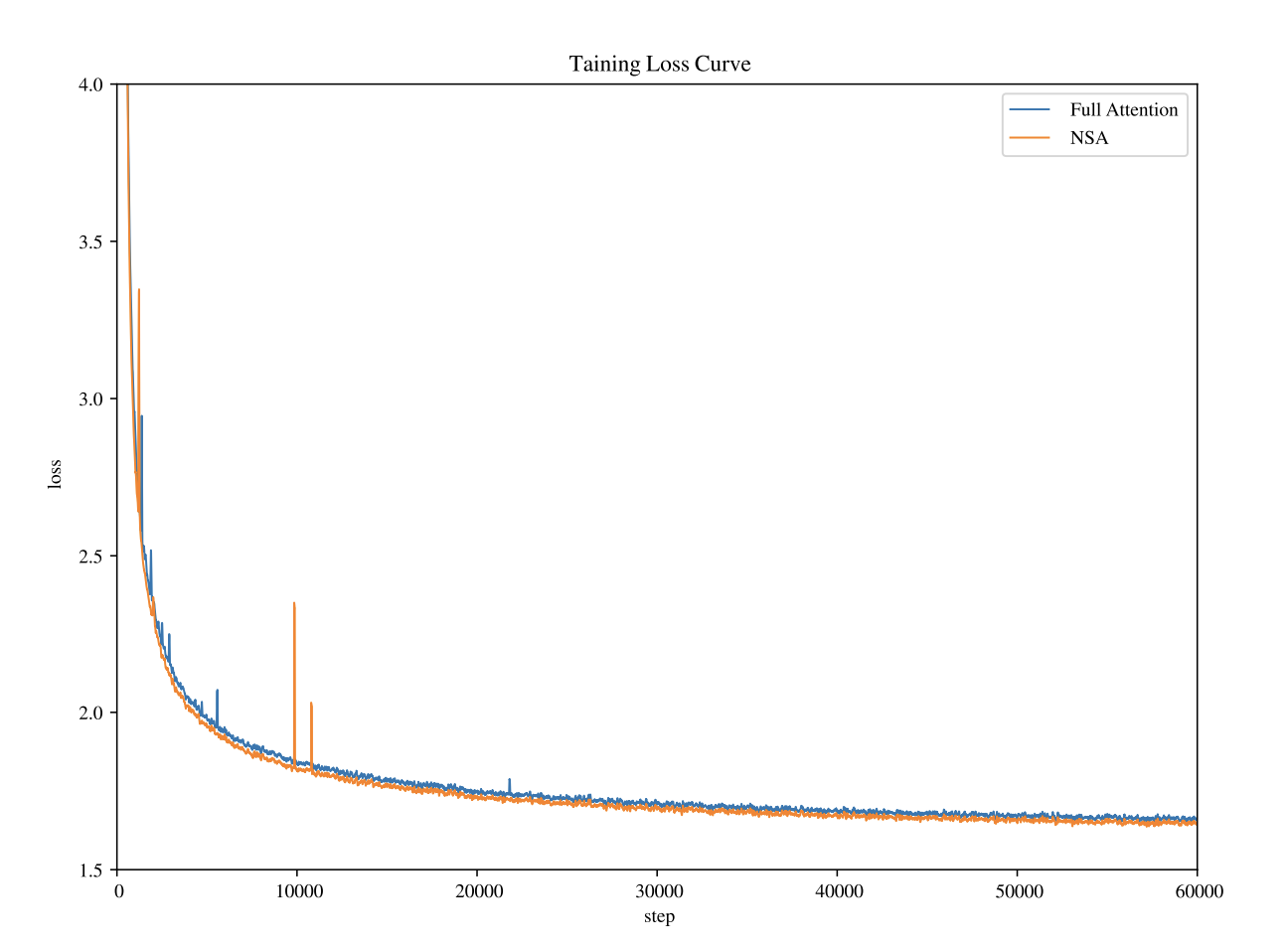
从 loss curve 可以发现比 full attention 还是缺了一些稳定性,但是 surprisingly 得到更低的 loss。看来是找到了正确的 inductive bias。
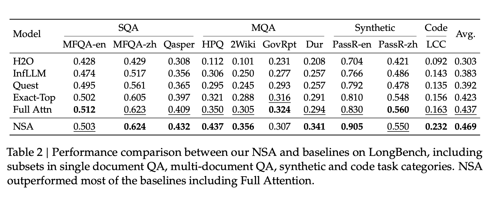
Benchmark 上超越了 full attention,在 Math & Coding 上有比较大的 margin。
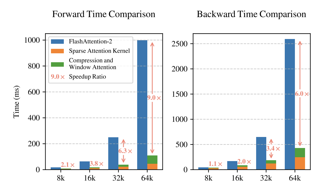
除此之外,同样是 Triton-based implementation,和 FlashAttention-2 比较,在 64K context length 下获得了 9 倍的 forward speedup & 6 倍的 backward speedup。比较橙色和绿色也发现不同的 mechanism 分配了很均匀的 latency。