ZHH-013
[Paper] Flow Matching for Generative Modeling
记号
- $p_0$: an easy distribution. You can imagine it as $N(0, 1)$ but not necessarily
- $q$: the target (data) distribution. We hope $p_1=q$. Note that we don’t know $q$ and we can only access it through samples.
- $\phi_t(x)$, where $x\in p_0$: the position of $x$ after time $t$
- $u_t(x)$: the real velocity field at time $t$.
- $v_\theta(x, t)$: 我们的神经网络, 希望它能够近似$u_t(x)$
Idea
我们的生成过程是求解ODE
\[\frac{dx}{dt}=v_\theta(x,t)\]其中,$v_\theta(x,t)$是神经网络。
训练目标“Flow Matching”指的是,我们试图构造一个flow $u_t(x)$,使得它满足这个条件;然后,我们用神经网络近似它:
\[L=\mathbb{E}_{t\sim \text{Uniform}(0,1)}\mathbb{E}_{x_t\sim p_t}\left[\left|v_\theta(x_t,t)-u_t(x_t)\right|^2\right]\]而这个$u_t(x)$的构造方式是通过conditional normalizing flow.
Conditional Normalizing Flow
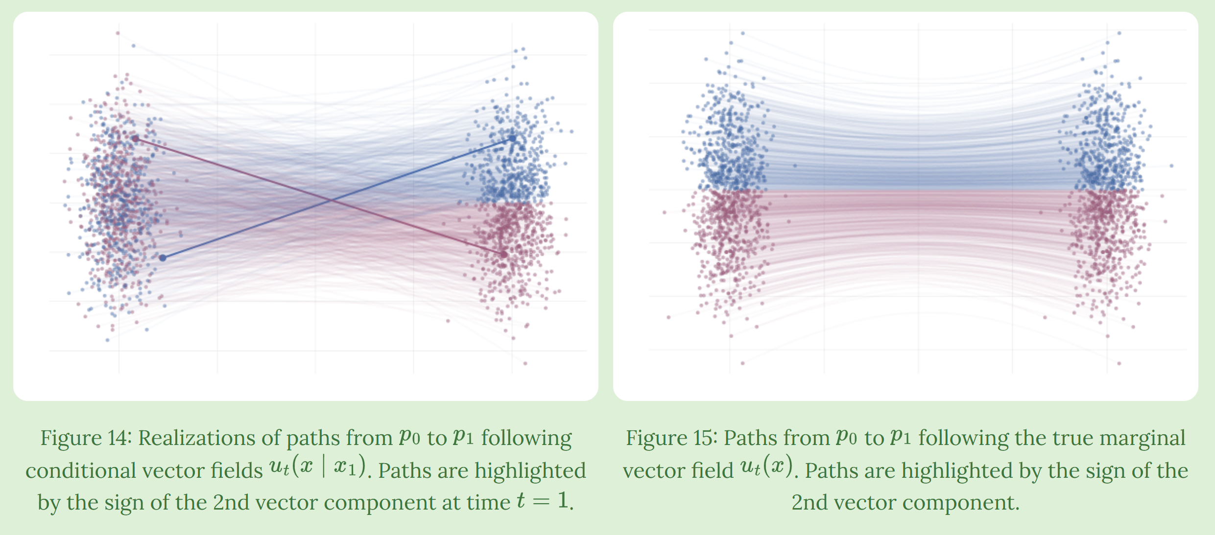
We define $p_t(x\mid x_1)$ (which we will design later) and set \(p_t(x)=\int p_t(x\mid x_1)q(x_1)dx_1 \tag{1}\) And we also define $u_t(x\mid x_1)$ as the conditioned velocity field.
- Here the intuition is that: $p_t(x\mid x_1)$ 可以看作表示了在 $t$ 时刻, 从 $x$ 出发最终走到 $x_1$ 的概率. (注意这个”概率”只是想象中的, 因为 flow 实际上是确定性的); 而 $u_t(x\mid x_1)$ 则是一个能和 $p_t(x\mid x_1)$ 对应上的 flow.
既然有了这样的 intuition, 我们自然应该有下面的性质:
- $p_1(x\mid x_1)$ 应当是一个 单点分布 (可以认为是一个 delta 分布或者是一个很小的高斯分布)
- 我们规定: $p_0(x\mid x_1)=p_0(x)$ (注意这样当然满足 $(1)$ 式)
- Intuition: 我们希望 $p_t(x\mid x_1)$ 是这二者的一个 interpolation. 在这样的人为设计下, 有很简单的构造方法. 其实我们就是利用了在 target distribution 是单点分布的时候很容易设计 interpolation 的性质.
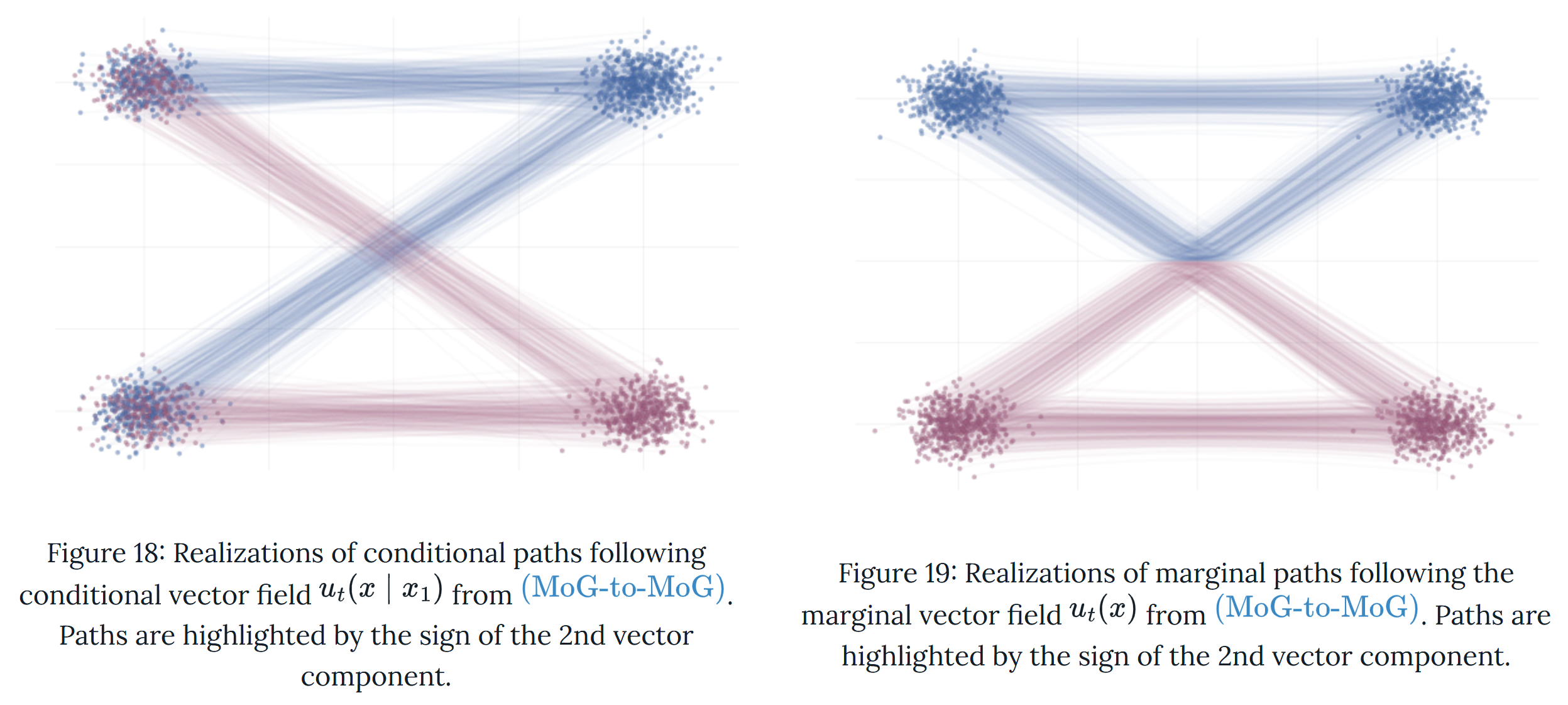
Theorem. If we set \(u_t(x)=\int u_t(x\mid x_1)\frac{p_t(x\mid x_1)q(x_1)}{p_t(x)}dx_1 \tag{2}\) 那么, 只要 $u_t(x\mid x_1)$ 能引出 flow $p_t(x\mid x_1)$, 那么 $u_t(x)$ 就是一个能引出 $p_t(x)$ 的 flow.
- Whether you care or not, I don’t want to include the proof. The intuition is simply a Bayesian rule.
这些操作的巧妙之处在于,虽然在我们的原训练目标中 $u$ 本身是intractable的 (涉及对数据集的积分), 但我们通过 condition 的方式可以重写 loss (差一个常数):
\[L=\mathbb{E}_{t\sim \text{Uniform}(0,1)}\mathbb{E}_{x_1\sim q}\mathbb{E}_{\epsilon \sim \mathcal{N}(0,1)}\left[\left|v_\theta(x_t,t)-u_t(x_t\mid x_1)\right|^2\right]\]直观理解: 最优的 $v_\theta(x,t)$ 就是 $u_t(x_t\mid x_1)$ 的一个加权平均; 实际上就是 $(2)$ 式.
$p_t(\cdot\mid x_d)$ 的设计
一个常见的方法是我们选择 \(p_t(x\mid x_d)=\mathcal{N}(\mu_t(x_d),\sigma_t(x_d))\)
它们必须满足 (其中 $\sigma_m=0$)
\[\mu_0(x_d)=0,\sigma_0(x_d)=1; \mu_1(x_d)=x_d,\sigma_1(x_d)=\sigma_m\]这个函数我们可以任意选取。这篇论文里选择了线性插值 (Optimal Transfer)
\[\mu_t(x_d)=tx_d,\sigma_t(x_d)=(1-t)+t\sigma_m\]以及对应关系
\[\phi_t(\epsilon\mid x_d)=\mu_t(x_d)+\sigma_t(x_d)\epsilon\]这对应的就可以很容易算出来
\[\phi_t(\epsilon\mid x_d)=t x_d+(1-t+t\sigma_m)\epsilon,\quad u_t(x_t\mid x_d)=x_d+\epsilon (1-\sigma_m) = x_d + \frac{1-\sigma_m}{1-t+t\sigma_m}(x_t-tx_d)\]In summary: The loss function is
\[\mathbb{E}_{t, x_1\sim q, \epsilon\sim N(0, I)} \|v_{\theta}((1-t)\epsilon+tx_1, t)-(x_1-\epsilon)\|^2\]Explanations
Diffusion 可以看作是一种 flow-matching, 只是采用了不同的 $p_t(\cdot\mid x_d)$ 的设计. Diffusion 对应的对应关系不是直线.
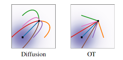
OT 可以在使用更少的步骤的情况下完成比 Diffusion 更好的生成效果.
Extensions
This part is from the blog Flow matching
Instead of conditioning on $x_1\sim q$, we can condition on anything you want.
In general, we can condition on a latent variable $z$ and try to write the loss function as
\[\mathbb{E}_{t, z\sim q(z), x_t\sim p(\cdot\mid z)} [\|u_{\theta}(t, x_t)-u_t(x_t\mid z)\|^2]\]In this way, we may have to:
- design $p_t(x\mid z)$
- design $u_t(x\mid z)$
- make the mathematics match the FM loss
- more…
举个例子: 我们可以 condition on $z=(x_1, x_0)$, and $p_t(x_t\mid x_1, x_0)=\delta (1-t)x_0+tx_1$ and $u_t(x_t\mid x_1, x_0)=x_1-x_0$ and $q(x_1, x_0)=q(x_1)p_0(x_0)$.
附录
更多内容,可以参考demo,包括一些推导和在toy dataset上的实现。